It’s no surprise to see disaggregated optical networks being widely adopted by data center providers. It’s an approach that fulfils their needs perfectly. Disaggregation triggers innovation, increases flexibility to mix and match best-of-breed networking components, avoids implementation lock-in and integrates into open source and commercial orchestration. What’s more, it accommodates the different lifecycles of various networking components. Line terminals, for example, usually follow a much shorter innovation cycle than optical line systems. 

It’s this key advantage that is now pushing disaggregation into the carrier space. Carriers can benefit from the latest and greatest technology without overhauling the entire infrastructure. They only need to replace the pieces that have undergone an innovation step. Typically that’s the line terminals, which have the shortest innovation cycle of about two to three years, driven by innovation in optical components, processors, new or enhanced modulation formats, components integration, etc.

Of course, carriers don’t usually build infrastructure from scratch. In most cases, they already have an installed base of various networking components. First of all the fiber, which defines some parameters, such as attenuation, dispersion, optical signal-to-noise rates, and as such potentially limits the maximum reach. Being the asset with the longest lifetime, fibers are not supposed to be replaced. A “bad fiber” can significantly impact reach.

With an average lifetime of about three to five years in the DCI space, and even more in a telecom environment, optical line systems remain in the network about twice as long as the terminals. Line systems deployed some years ago might still use fixed grids of, for example, 50GHz. If this has been deployed several years ago it could potentially limit the channel baud rate.

Coherent channel bit rates can be realized by adjusting the spectrum and/or the modulation format, depending on the available spectrum and distance. The picture below shows the options for 300Gbit/s.

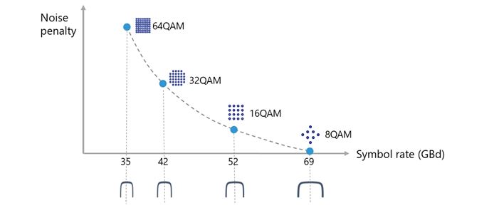
Increasing the symbol rate (higher QAM values) goes hand-in-hand with an increased noise penalty, limiting the distance. Higher baud rates might not match with existing filters.

Usually, these channel bit rates are achieved in discrete steps, as highlighted by the dots in the graph. There are significant performance steps between QAMs, which impacts reach, and significant bandwidth steps between QAMs, which impacts filtering. 

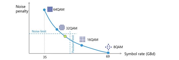
The figure below extends this explanation to multiple channel bit rates from 100Gbit/s to 600Gbit/s, displayed in steps of 50Gbit/s. Each dot represents an option to realize a given channel bit rate. The higher the channel rate you want to achieve, the more limited you become with distance and spectrum: While distance and spectrum might not impact lower bit rates, higher bit rates might not be able to run over longer distances and through filters using “thinner” grids.

With our FSP 3000 TeraFlex™, we’re softening these boundaries / discrete steps, so the required channel bandwidth can be realized through a flexible combination of fractional QAM capabilities (which allows a flexible mix of two adjacent modulation formats, e.g., from 0% 16QAM and 100% 8QAM to 100% 16QAM and 0% 8QAM) and continuous bandwidth setting for close adaption to filter passbands (so the signal fits into any spectrum).

This allows us to make use of each and every option along the channel rate curves above, which gives far more choices, especially in areas where the curves show a steeper shape.

This translates into the following benefits: 

• In a given environment, where the reach and filters are defined and cannot be changed, we can realize higher channel bit rates (as shown below). With discrete modulation steps and baud rates, a 300Gbit/s channel cannot be realized in the given environment, limited by reach and filter. With fractional QAM enabling ultra-flexible modulation, there are several options for a 300Gbit/s channel to run through the given environment. (E.g., a 50GHz grid and a given distance might only allow for 200Gbit/s channels if we use discrete steps. However, with ultra-flexible modulation we can use 300Gbit/s channels as well.) Of course, 300Gbit/s is just an example. The same principle applies for higher channel rates all the way up to 600Gbit/s

This can create a significant increase in the total capacity transported over a given network, lowering the cost per Gbit mile in brownfield scenarios. A fixed grid structure is no longer a barrier to growth.

• For a given channel bit rate we can increase the reach (by moving from left to right along the curves). So we’re able to bridge longer links, going from metro to regional to long-haul to even the distances required for submarine links – depending, of course, on the channel bit rate. 

In summary, our TeraFlex™, is not only a preferred option in greenfield and data center interconnect scenarios, it enables existing deployments to be optimized in terms of capacity and distance, significantly reducing total cost of ownership.